Environment
The Environment screen shows you everything R is holding in memory. Instead of typing ls() or str() in the console to check on your variables, you can switch to Environment and see names, types, sizes, and previews at a glance.
Overview
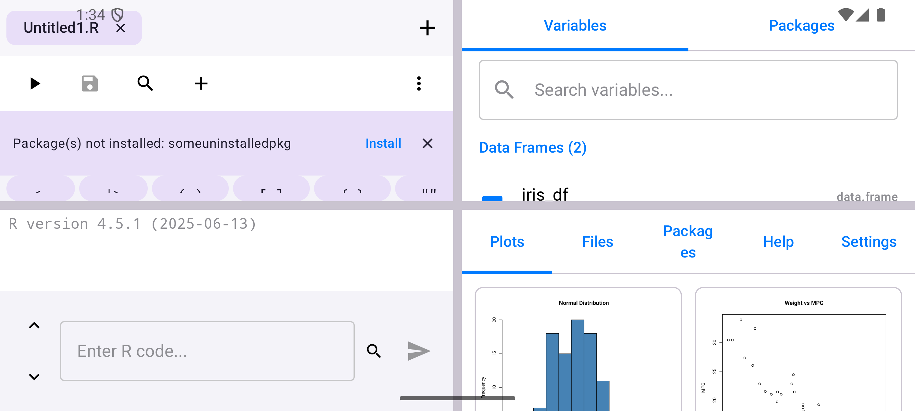
The Environment screen has the following layout:
- Title bar showing “Environment” with a memory badge (e.g., “15 KB”), a refresh icon, and an overflow menu (see Environment Menu)
- Two tabs: Variables and Packages
- Search bar with a magnifying glass and “Search variables…” placeholder
- Variable list grouped by type, with each entry showing a type icon, name, value preview, class, and memory size
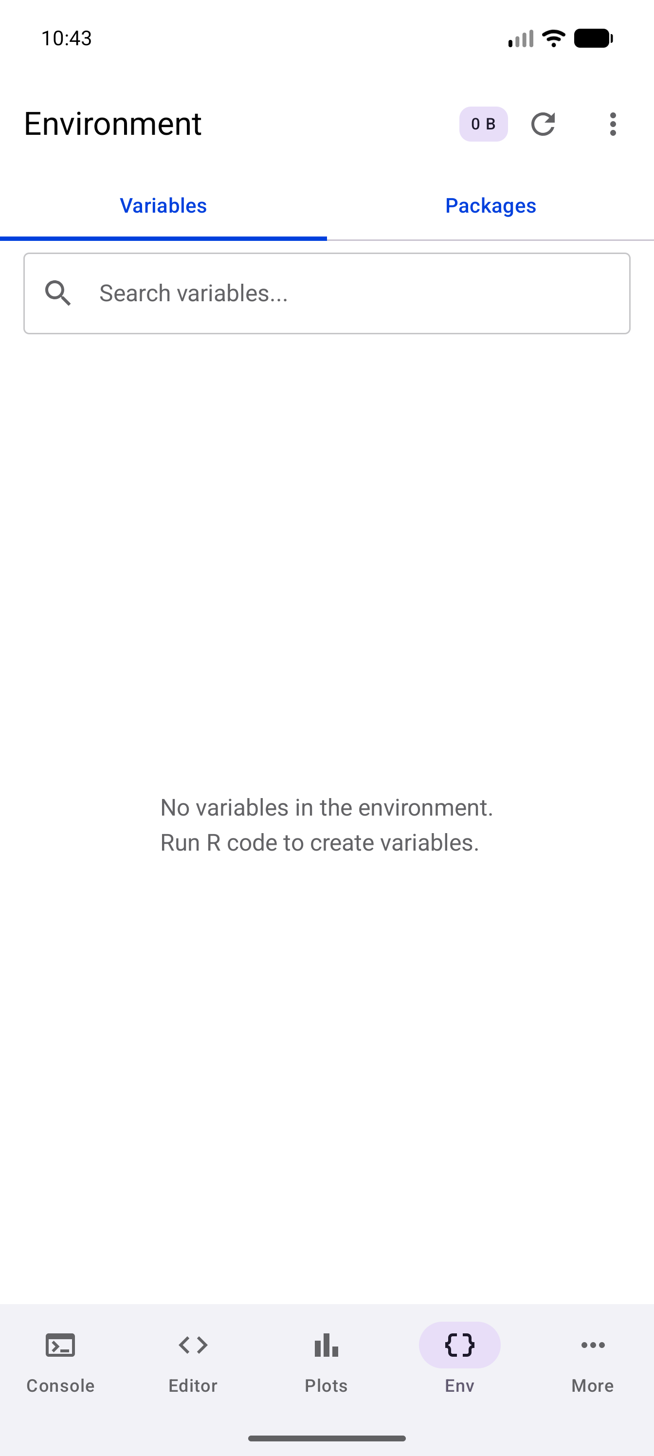
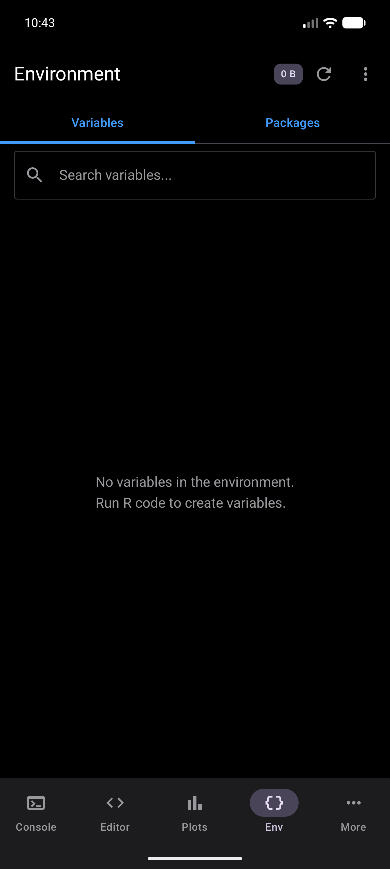
Before you run anything, the screen is empty and tells you so:
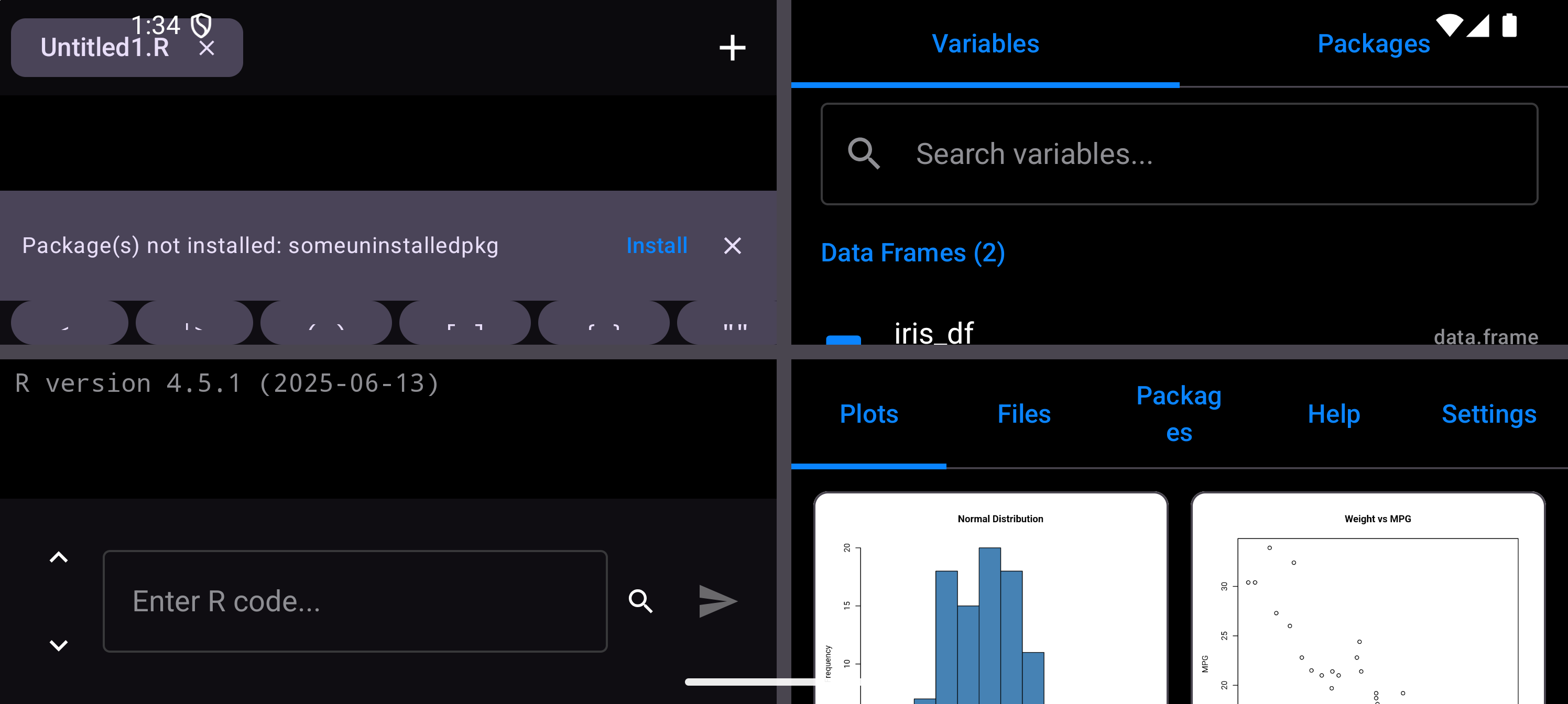
Once you have created some variables it fills in:
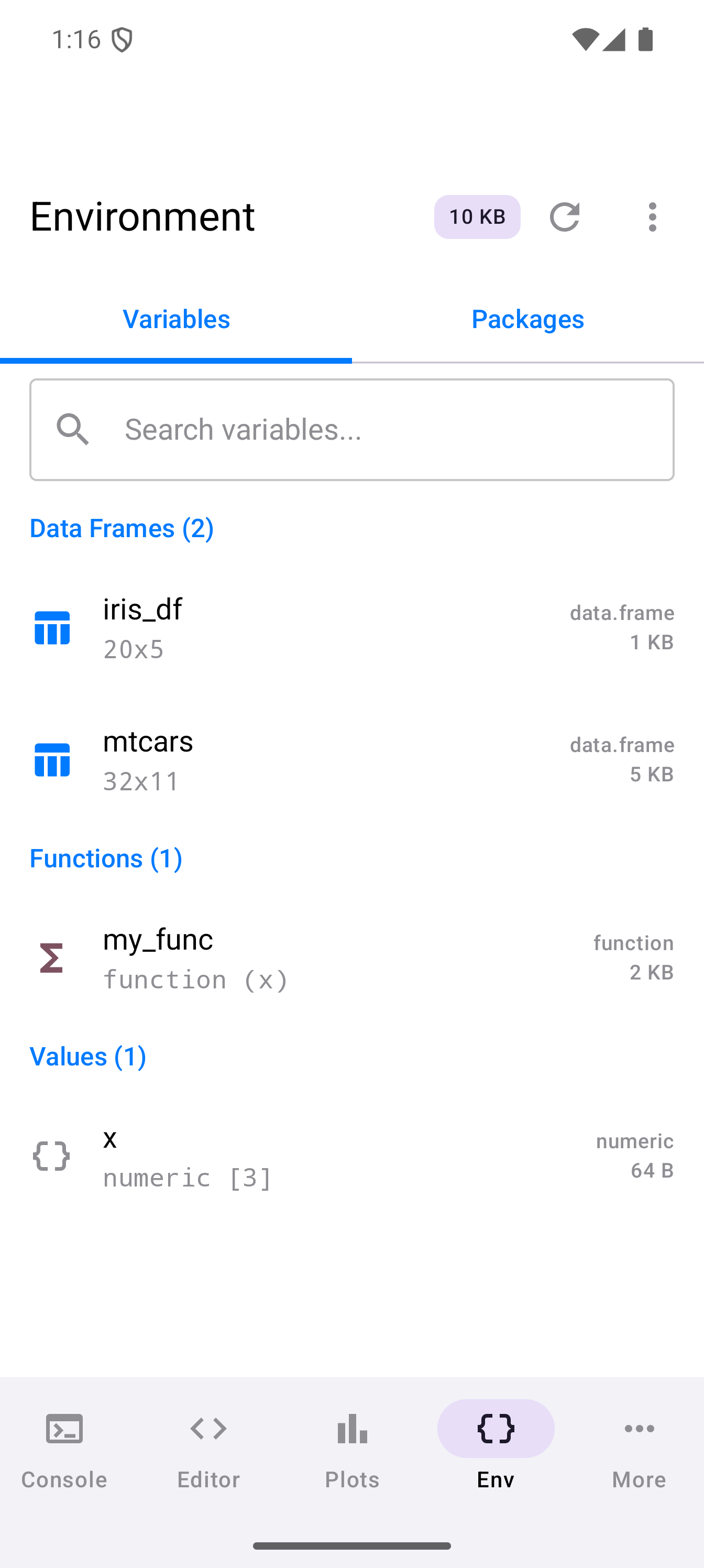
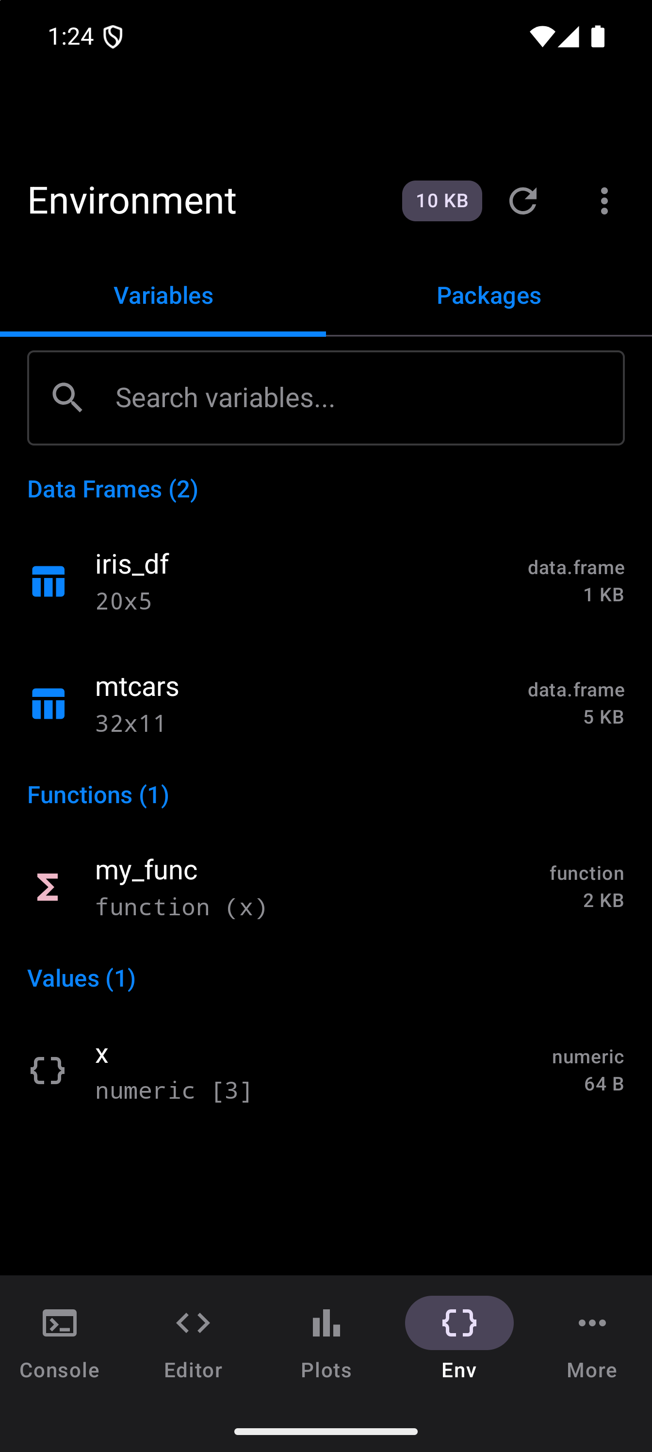
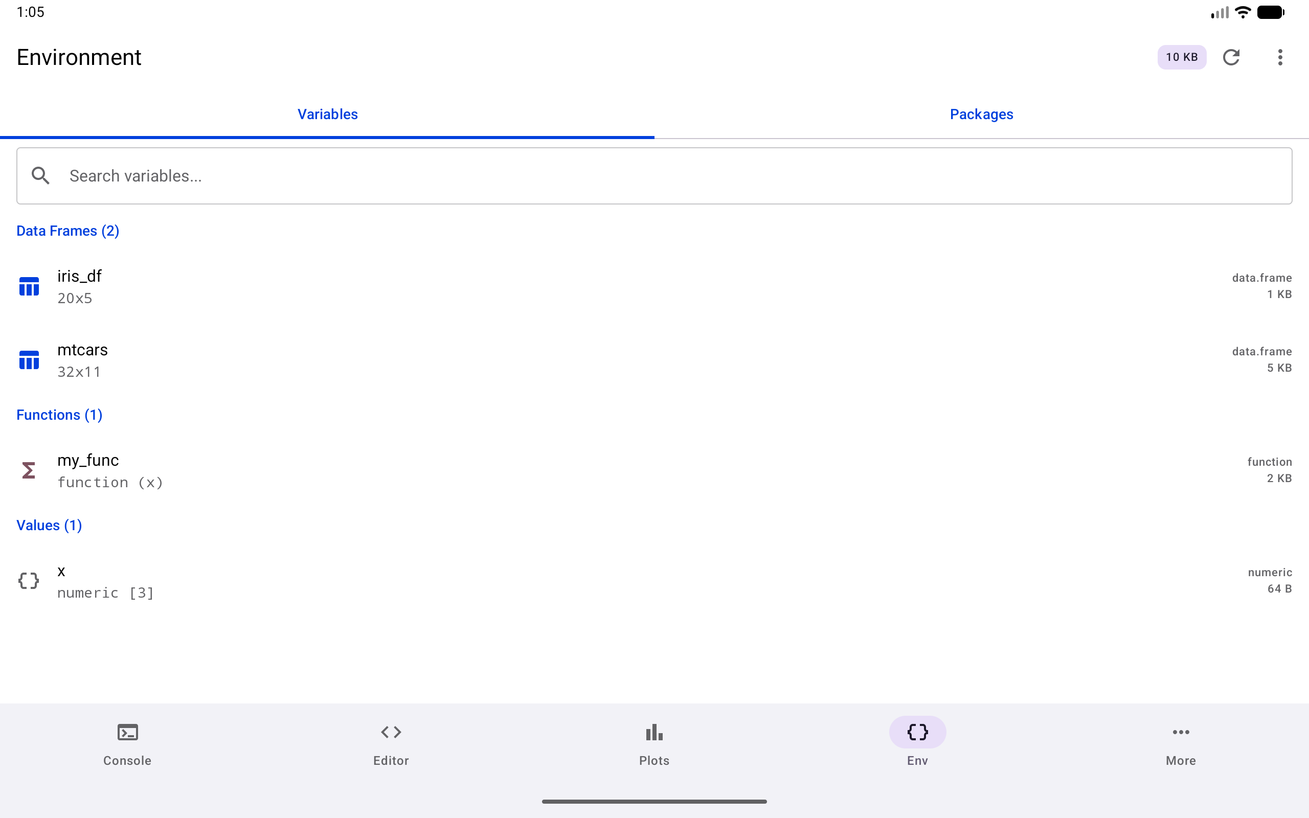
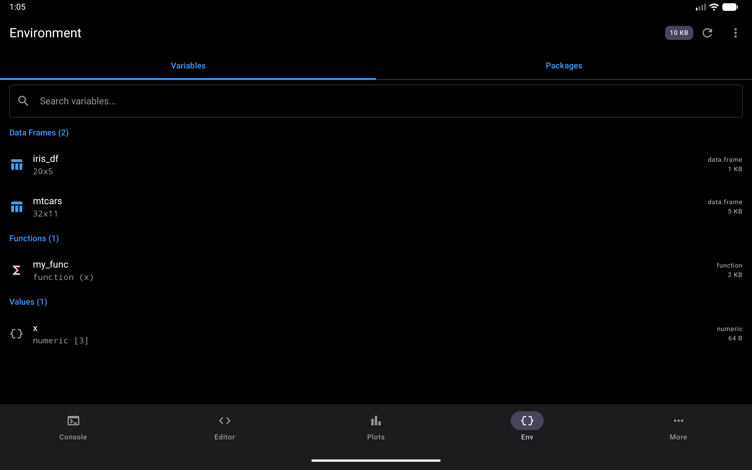
The memory badge in the title bar updates as you create and remove variables, giving you a running total of how much memory your workspace is using.
Variables Tab
The Variables tab is the default view. As you create variables in the Console or Editor, they appear here automatically. The list is read from R when the screen opens and again each time a command in the Console or a run from the Editor finishes; the refresh icon reads it at once. It is not read while R is busy, so a long computation is never kept waiting by it. After a command that ran past the time limit, the list waits until R finishes that command, or until Check Again on the Console’s banner finds R answering.
Variables are grouped into sections by their R type, in this order on screen: Data Frames, Matrices, Lists, Functions, then Values.
- Data Frames: includes
data.frame,tibble, anddata.tableobjects. Each entry shows the name, dimensions (e.g., “32x11”), class (data.frame), and memory size (e.g., “7 KB”). A table icon appears on the left. - Matrices: matrices and arrays. Each entry shows the name, its class and dimensions (e.g., “matrix [3x4]”), and size. A grid icon appears on the left.
- Values: scalars, vectors, strings, logicals, and other simple objects. Each entry shows the name, a value preview (e.g., “42”), class (
numeric), and size (e.g., “56 B”). A braces icon appears on the left. - Functions: any custom functions you have defined. Each entry shows the name, function signature, class, and size. A sigma icon appears on the left.
- Lists: nested list structures. Each entry shows the name, a summary like “List of 3”, class, and size. A list icon appears on the left.
Each section header shows a count in parentheses (e.g., “Data Frames (2)”) so you can quickly see how many objects of each type you have.
Watch List
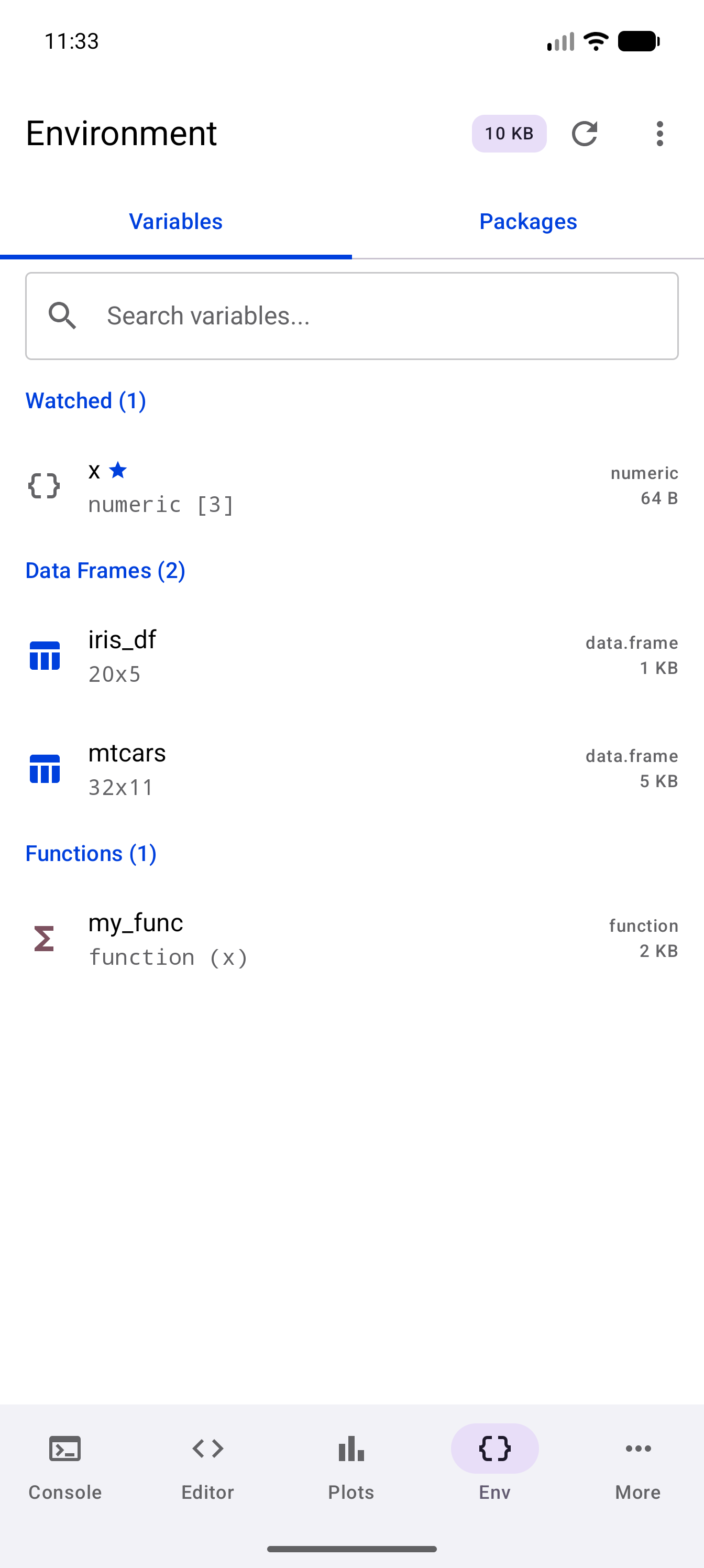
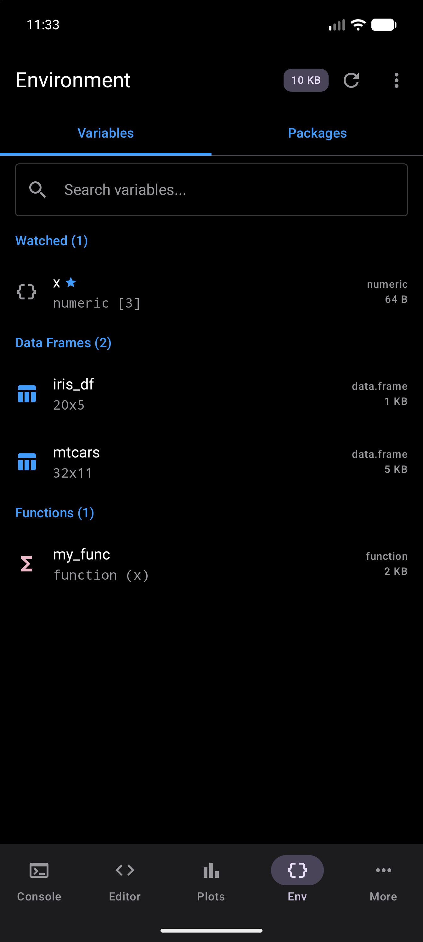
The watch list lets you pin important variables to the top of the Environment so they stay visible no matter how many other objects you create. Watched variables appear in their own “Watched” section above the type-based groups.
Adding a variable to the watch list
- Long-press any variable in the list to open the context menu (with a mouse or trackpad, right-click it).
- Tap Watch.
- The variable moves to the “Watched” section and displays a star icon next to its name.
Removing a variable from the watch list
- Long-press the watched variable.
- Tap Unwatch.
- The variable returns to its normal type-based group.
Clearing the entire watch list
- Tap the overflow menu (three-dot icon) in the Environment title bar (see Environment Menu).
- Tap Clear Watch List.
- All variables are unwatched and return to their standard groups.
Watching is especially useful during debugging or data-cleaning workflows where you need to keep an eye on a handful of key variables while the rest of your workspace grows.
Variable Details
Long-press any variable, or right-click it with a mouse or trackpad, to open its menu of quick actions. Here is the menu for the iris_df data frame:
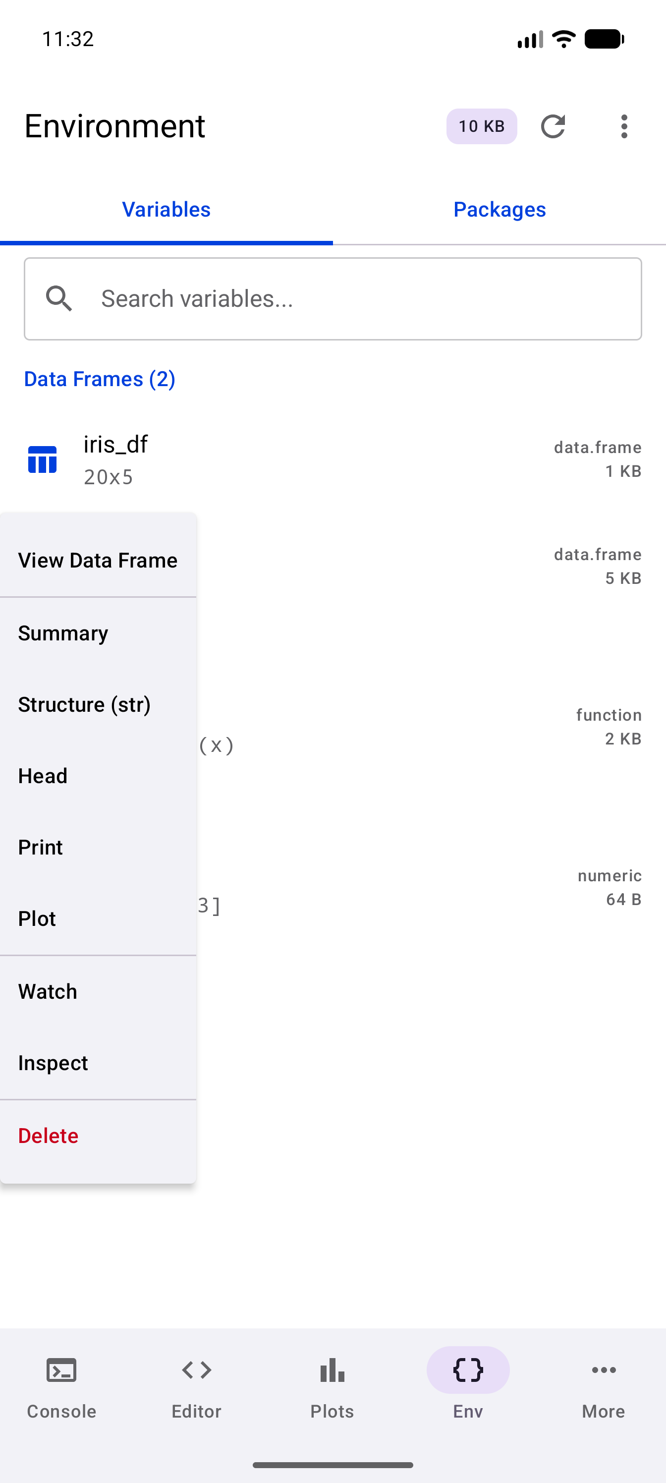
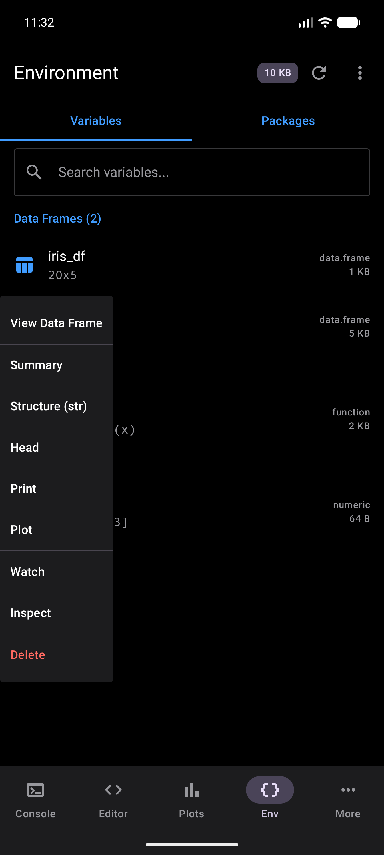
The quick actions let you run common inspection commands without switching to the Console:
| Action | What it does |
|---|---|
| View Data Frame | Opens the Data Frame Viewer (data frames only) |
| Summary | Runs summary() and shows the result |
| Structure (str) | Runs str() to show the internal structure of the object |
| Head | Runs head() to show the first few rows or elements |
Runs print() for the full output |
|
| Plot | Runs plot() for a quick plot (not offered for functions) |
| Watch or Unwatch | Adds the variable to the watch list, or takes it off |
| Inspect | Opens the detail sheet described below |
| Delete | Removes the variable from R’s memory |
These quick actions are especially useful for data frames. You can check column types with Structure (str), glance at the first rows with Head, or get summary statistics with Summary, all without typing a single command.
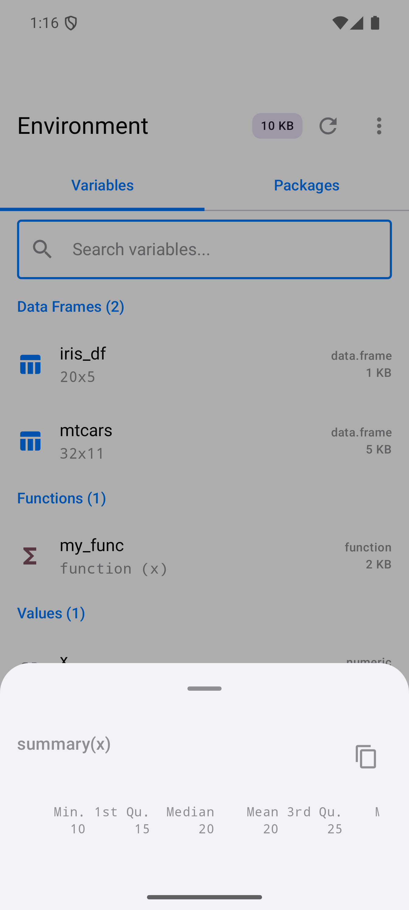
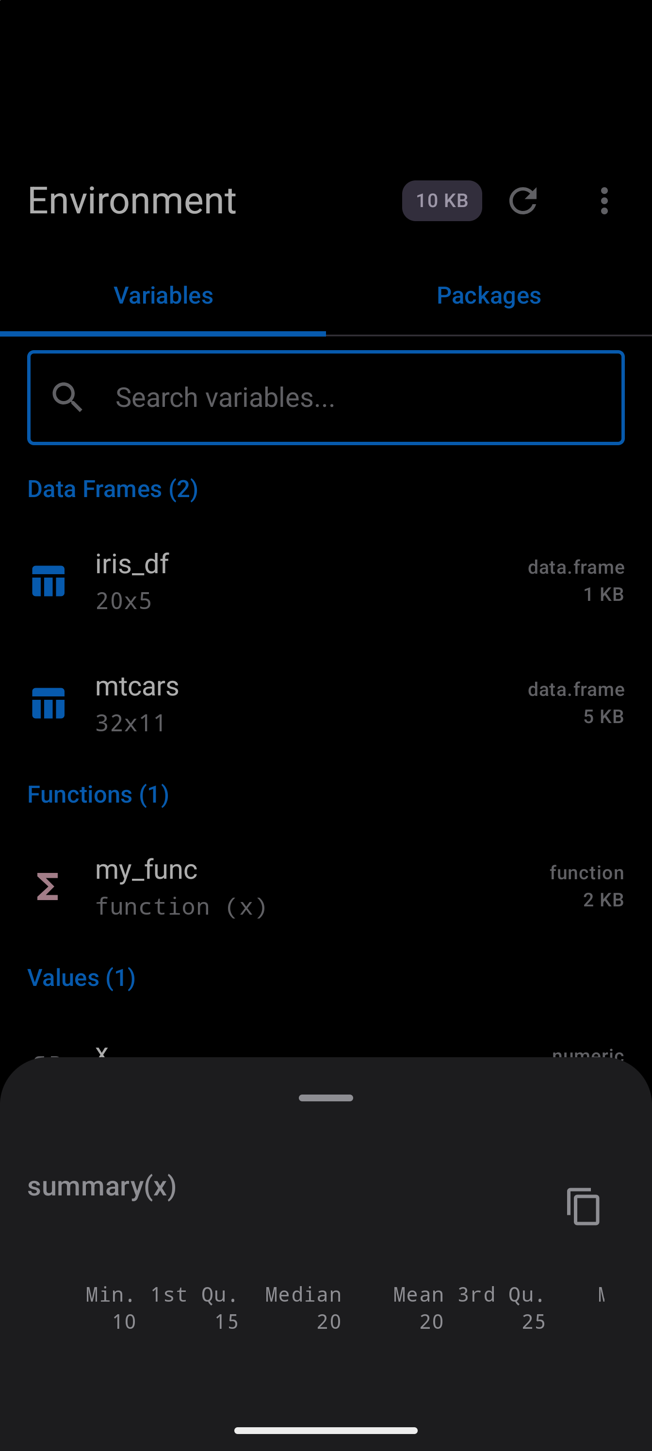
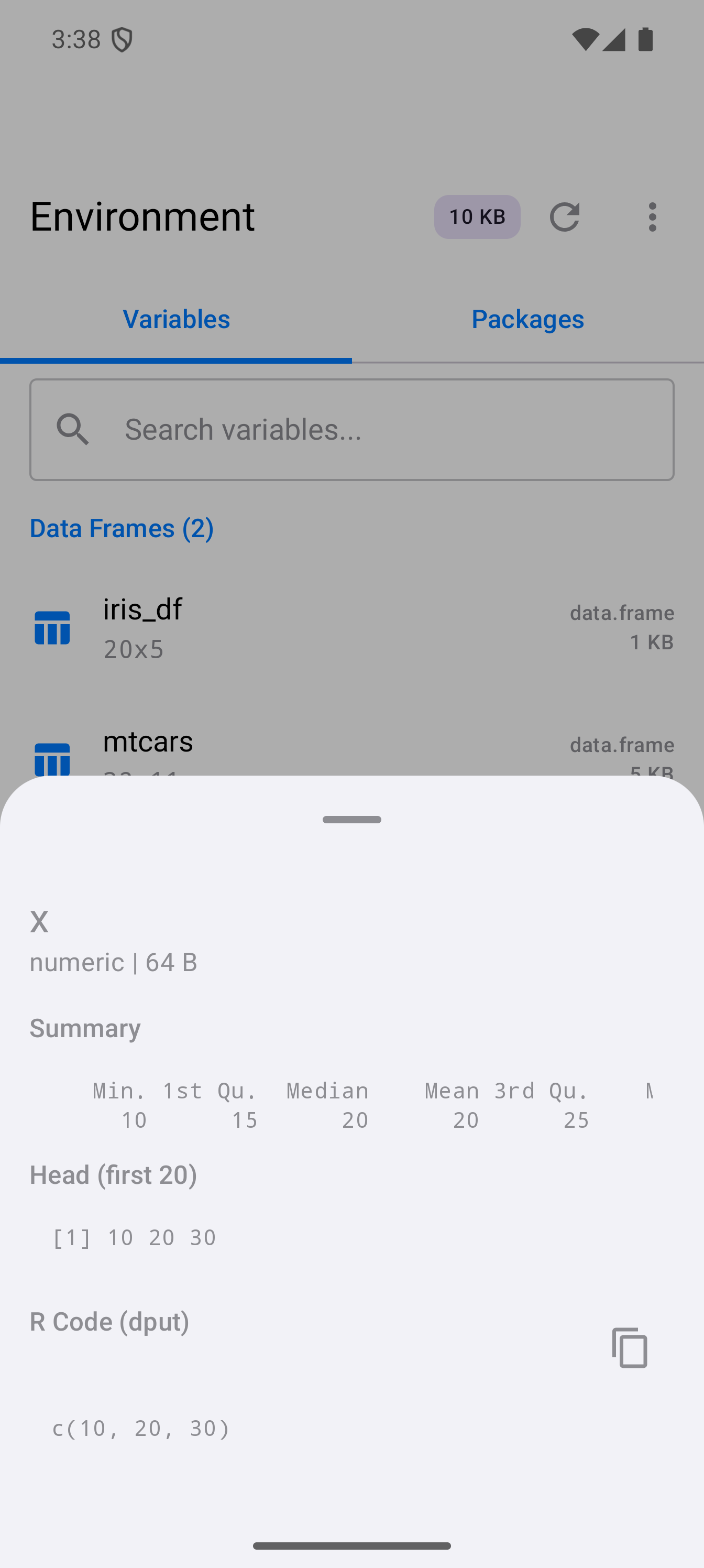
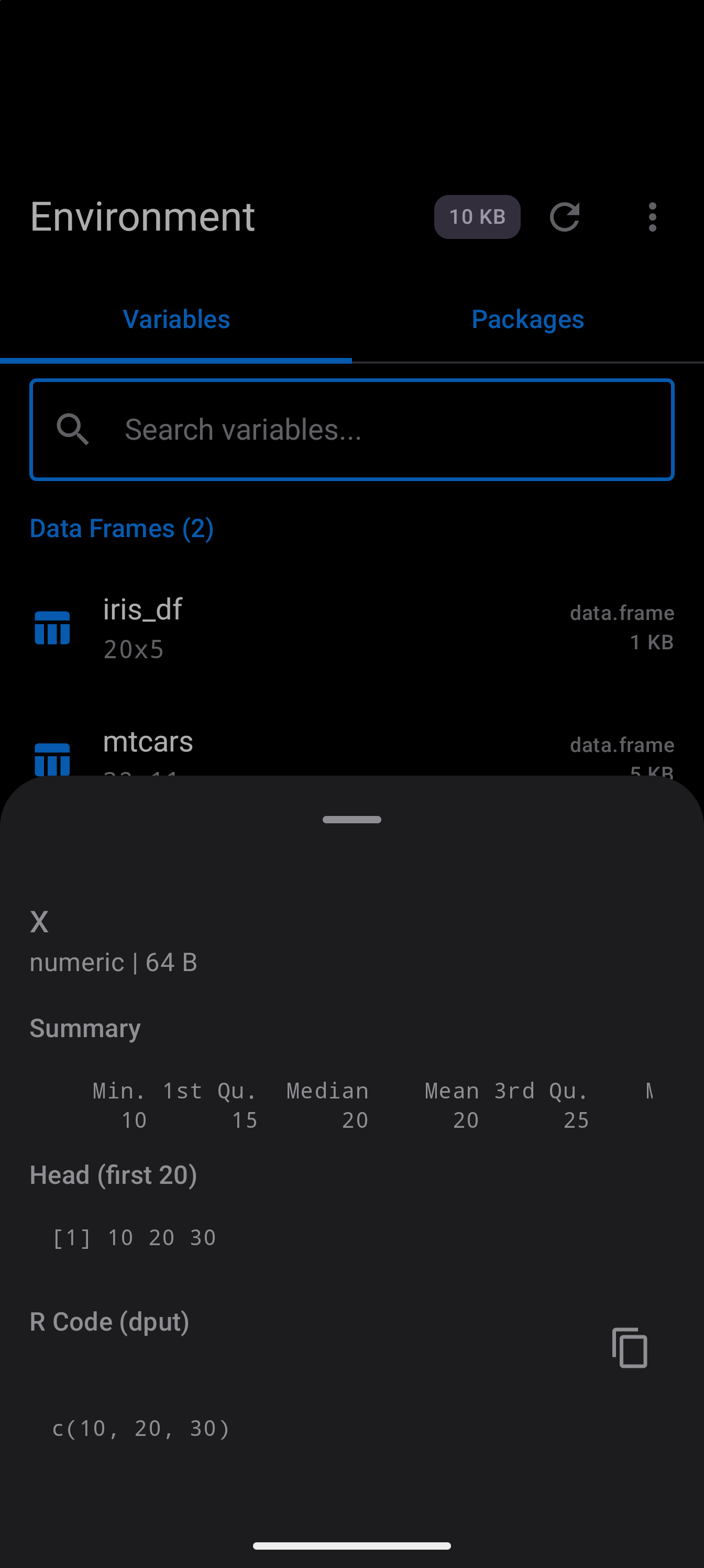
Tap any variable, or choose Inspect from its menu, to open a detail sheet with its class, size and structural information. For data frames this includes the dimensions, a preview of the first 10 rows and an Open in Data Frame Viewer button; for functions, signatures and bodies; for vectors, summary and head output. Below that is the object’s dput() code, with a button to copy it.
Data Frame Viewer
For data frames, you can open a full-screen modal viewer that presents your data as a scrollable table. This gives you a spreadsheet-like view where you can:
- Scroll horizontally and vertically through all rows and columns
- See column headers with their types
- Inspect individual cell values
To open the viewer, long-press a data frame variable in the variable list and choose View Data Frame from the context menu, or tap it and choose Open in Data Frame Viewer on its detail sheet. After an import, View Data on the wizard’s Imported screen opens the new data frame here too (see Data Import Wizard). This is much more practical than printing large data frames to the console.
If you need to load data from Excel files, CSV files, or databases, install the appropriate packages first. See the Packages guide for details on installing packages like readxl, readr, or DBI.
Column details
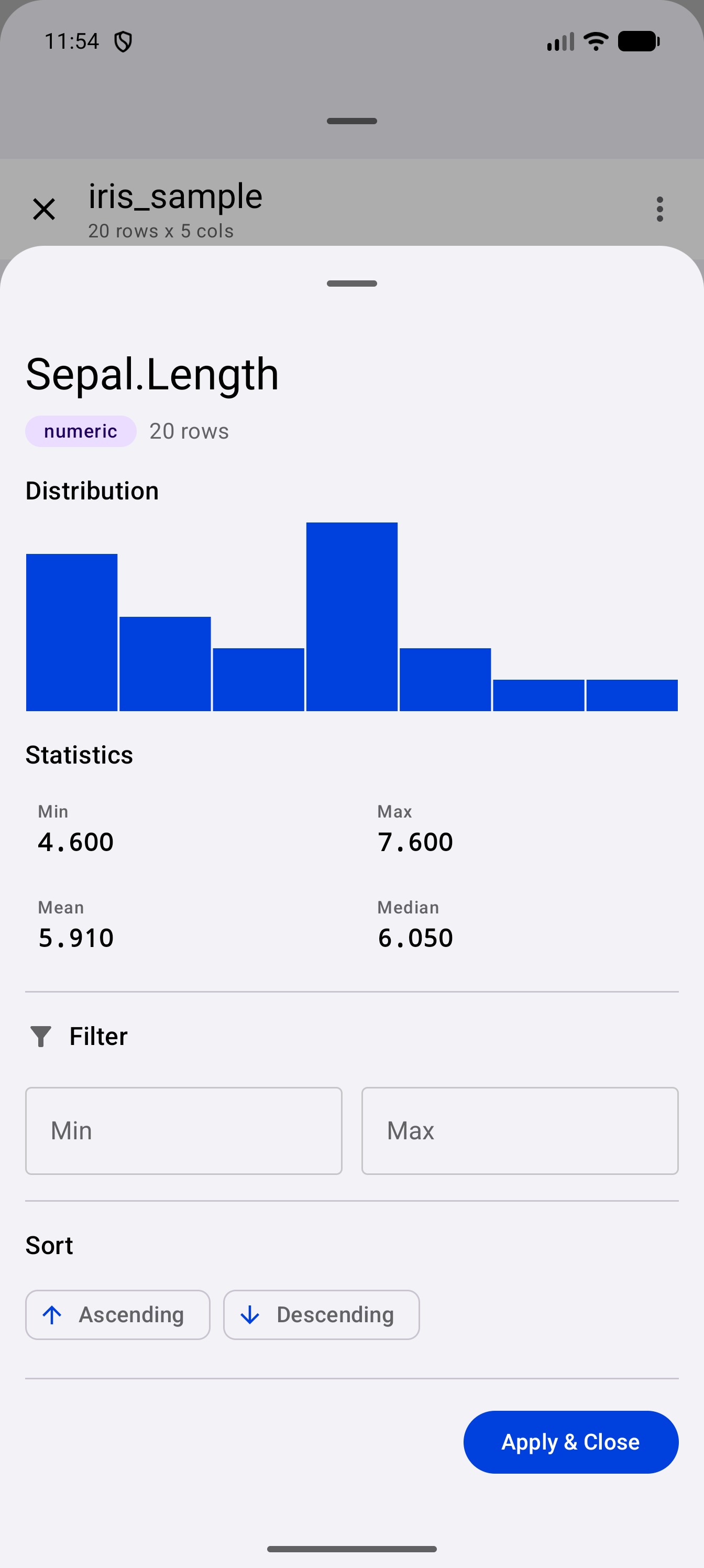
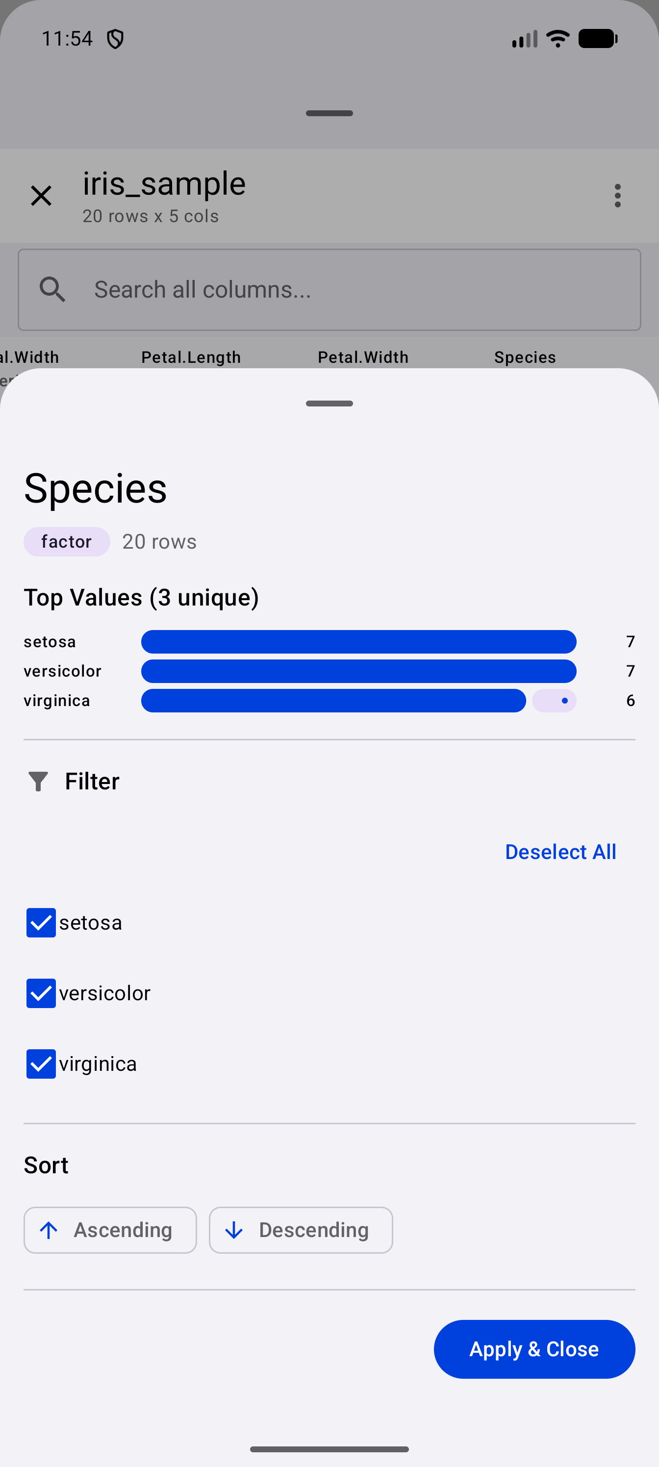
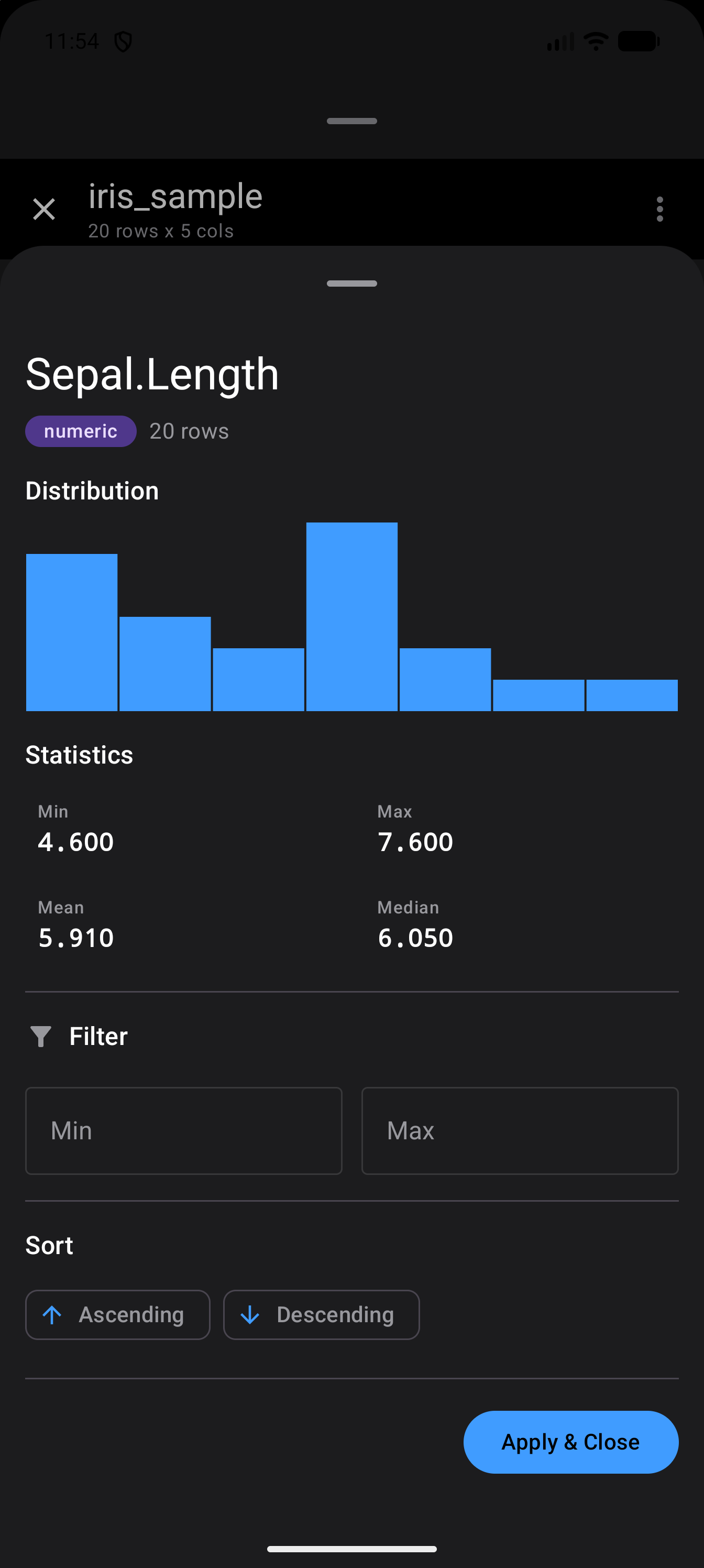
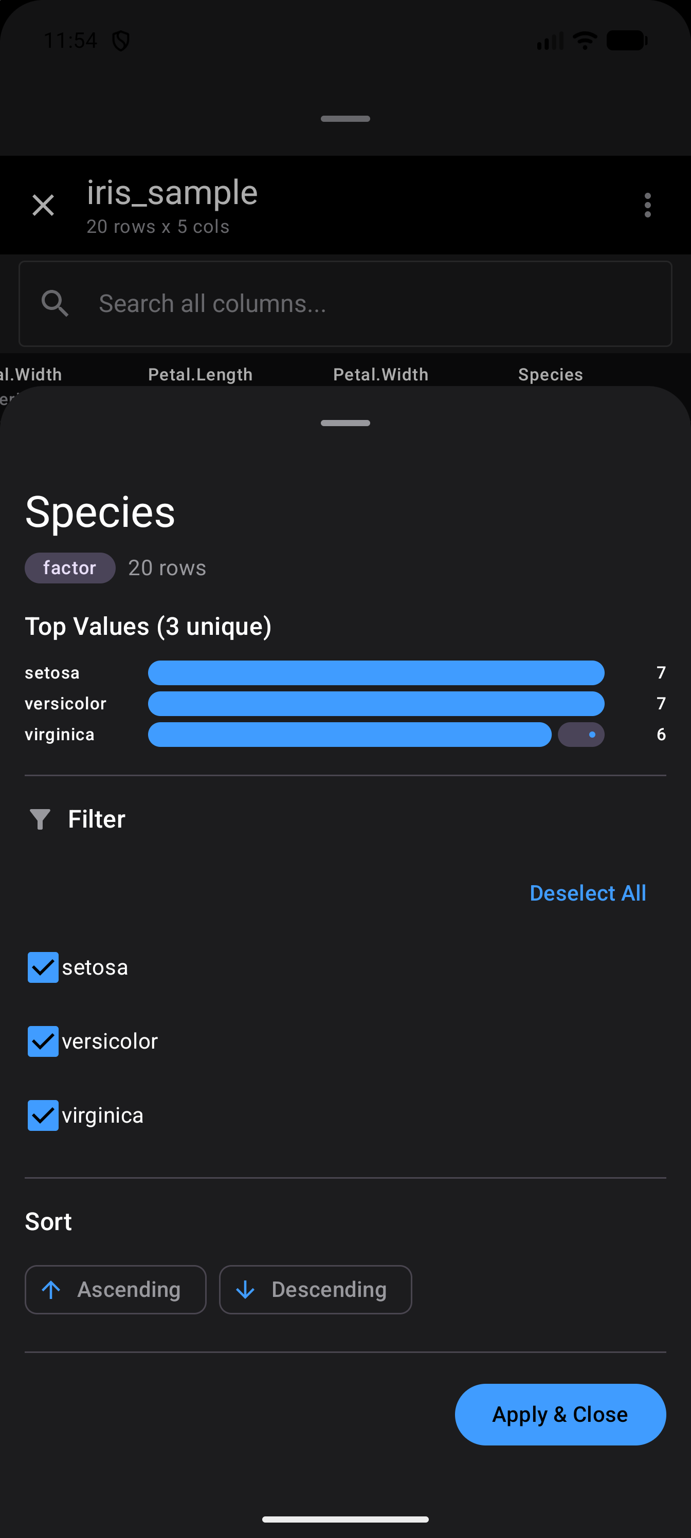
Long-press a column header, or right-click it with a mouse or trackpad, to open its detail sheet. The sheet shows:
- Type badge and row count, plus the number of NAs when the column has missing values
- Distribution chart: histogram for numeric columns, frequency bars for categorical columns, TRUE/FALSE bar for logical columns
- Statistics (numeric only): min, max, mean, and median
- Filter controls adapted to the column type (range for numeric, checkboxes for categorical, search for high-cardinality text, toggles for logical)
- Sort buttons: Ascending and Descending, plus Clear Sort once the grid is sorted by this column
When you are done, tap Apply & Close to go back to the grid. If the column has a filter, a Clear Filter button beside it takes that filter off. Here are the sheets for a numeric column and a categorical one:
Missing values and large data frames
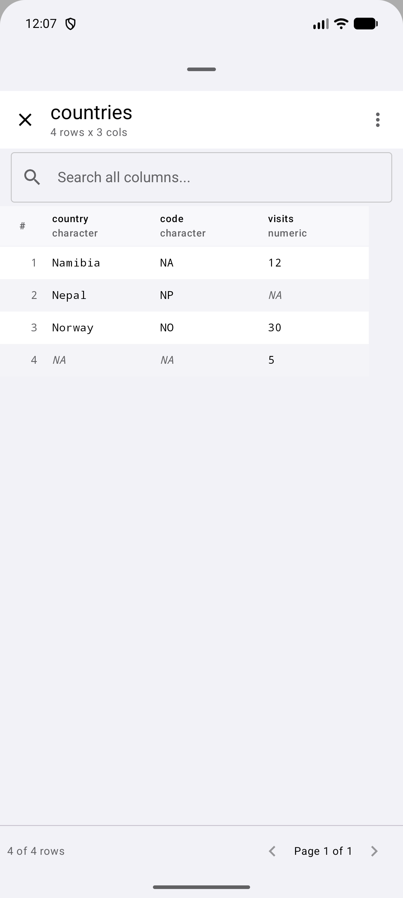
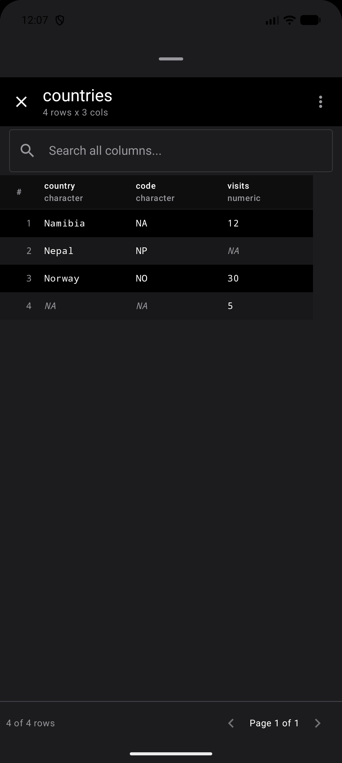
A missing value is drawn as NA in italics and a muted color, so it stands apart from a cell that holds the text “NA”. TalkBack reads it as “missing”. In this small data frame, Namibia’s country code is the text “NA”, in plain type, and the other three NAs are missing values:
The viewer holds at most one million cells. A larger data frame loads its first rows up to that limit, and a note above the grid says how many of the total it is showing. Search, filters, sort and export work on those rows; Copy View as R Code covers every row, because it runs in R.
Exporting and copying
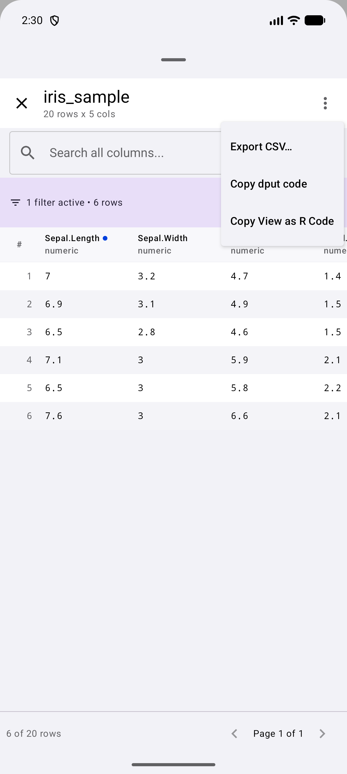
The three-dot menu in the viewer’s title bar offers:
- Export CSV… saves the rows the grid is showing, with your search, filters and sort applied, as a CSV file wherever you choose through Android’s file picker.
- Copy dput code copies the
dput()of the whole data frame, ready to paste into a question or a bug report. - Copy View as R Code appears once you have sorted or filtered, and copies R code that produces the same view from the data frame in your workspace.
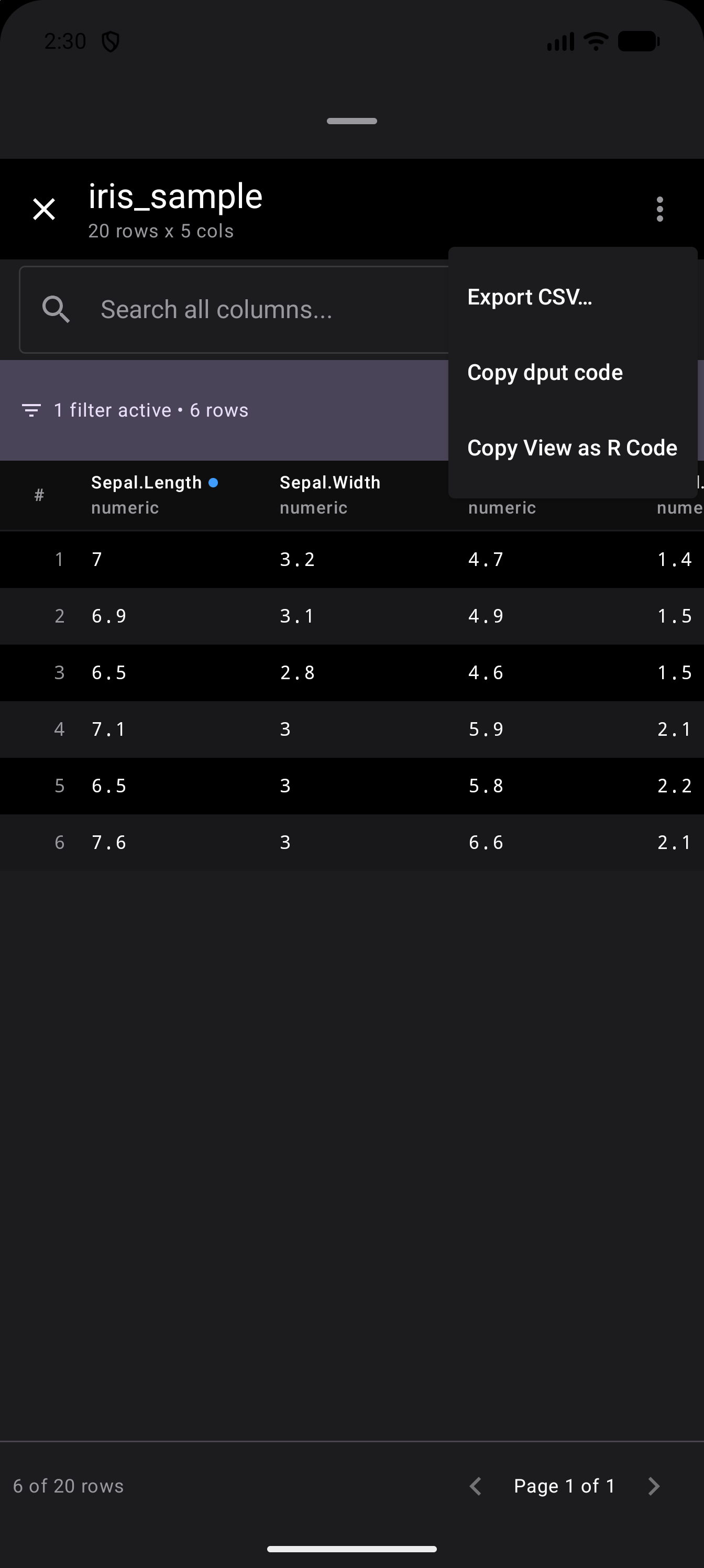
While a filter is on, a bar above the grid says how many filters are active and how many rows are left, and Clear All at its right end takes every filter off. A dot beside a column’s name shows that the column is filtered. Here a filter on Sepal.Length keeps 6 of the 20 rows, and the menu is open:
Comparing Data Frames
Compare Data Frames shows two data frames together in one grid and tints what is different between them. It is a handy way to check what a step of your data cleaning did, such as fixing some values or rounding a column.
To open the comparison view:
- Tap the overflow menu (three-dot icon) in the Environment title bar (see Environment Menu).
- Tap Compare Data Frames.
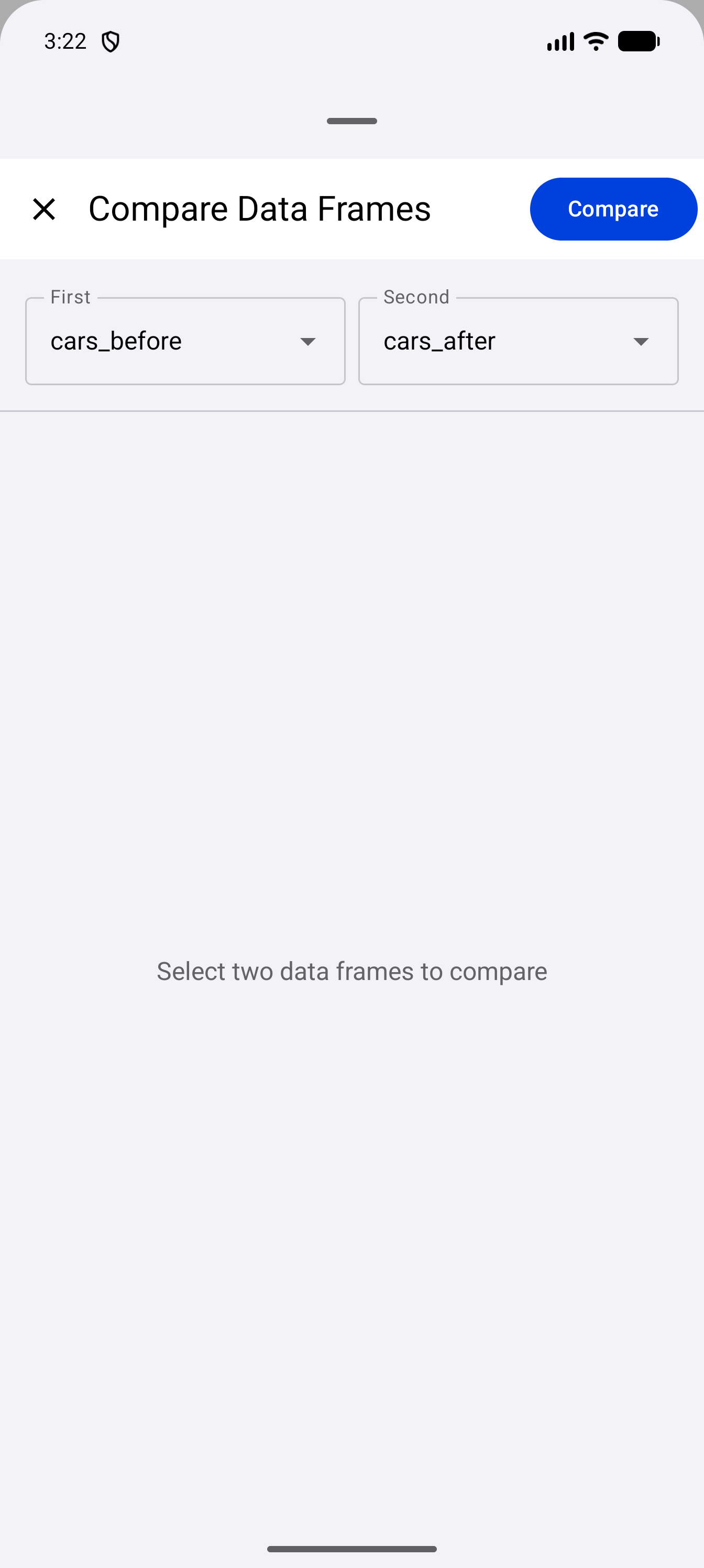
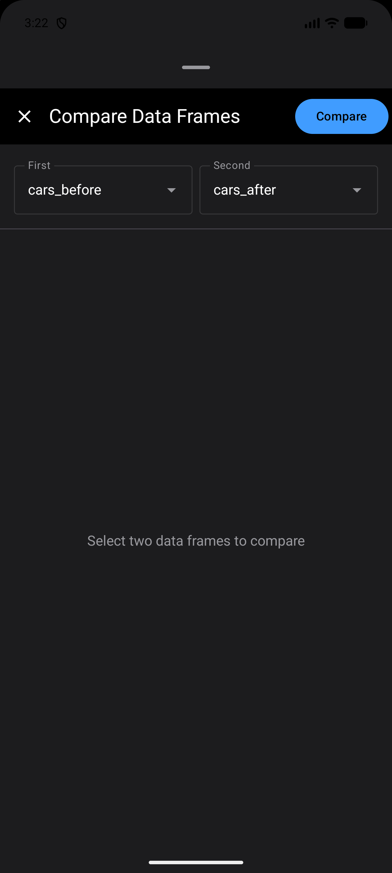
- In the comparison sheet, select the first data frame from the First dropdown and the second from the Second dropdown. Both dropdowns list all data frame objects currently in your workspace.
- Tap Compare, at the top right of the sheet, to run the diff.
To try it yourself, run this in the Console. It makes two small data frames from mtcars, where the second has one more row than the first and one changed value:
cars_before <- head(mtcars[, 1:3], 5)
cars_after <- head(mtcars[, 1:3], 6)
cars_after$mpg[2] <- 23.5
Then pick cars_before as First and cars_after as Second. Here is the sheet before and after tapping Compare:
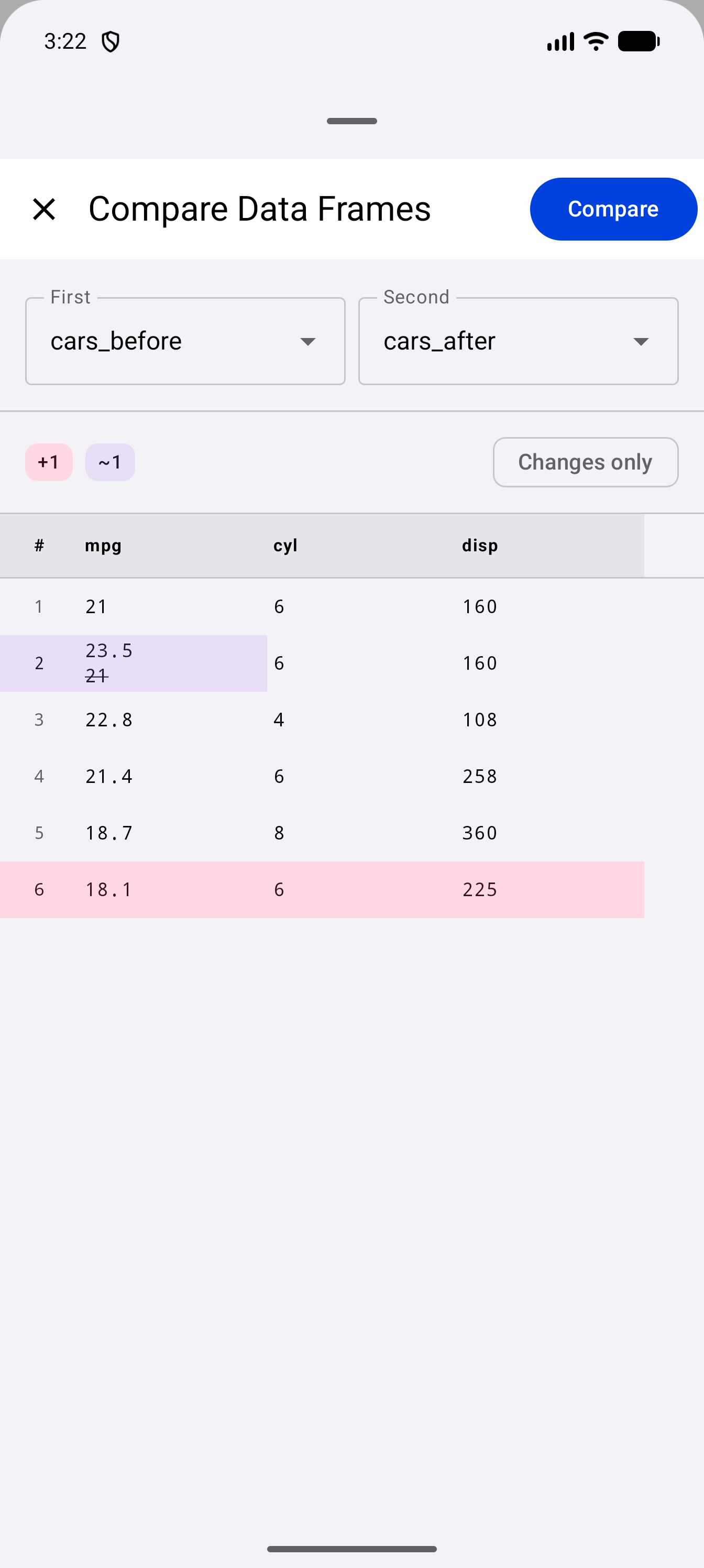
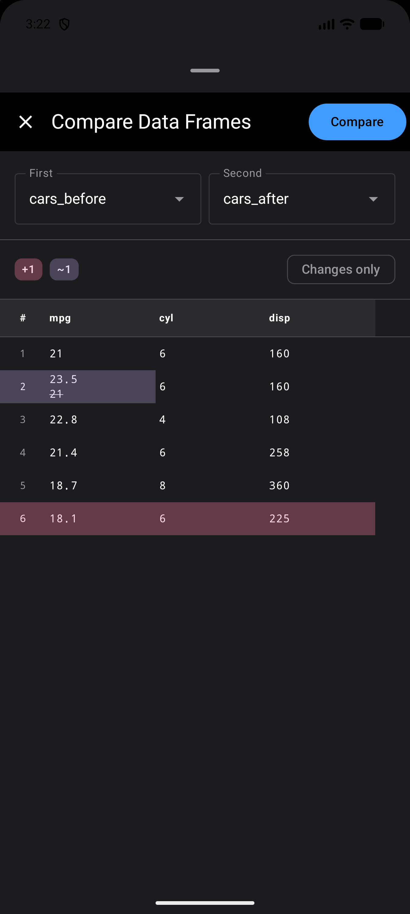
The results appear as a grid you can scroll up, down and sideways. The first column holds the row numbers. Anything that differs is tinted:
- A row or a column that is only in the second data frame is marked as added, with a pink tint.
- A row or a column that is only in the first data frame is marked as removed, with a red tint.
- A cell whose value is different is marked as modified, with a purple tint. It shows the new value on top and the old value crossed out below it.
- Cells that are the same in both have no tint.
The row number is tinted too, so you can see at a glance which rows have a change. TalkBack reads each tinted cell, row number and column name with “added”, “removed” or “modified” after it. For a modified cell it also reads the old value, such as “5, modified, was 4”.
A summary bar above the grid counts the changes: +2 means two rows added, -1 one row removed, ~5 five rows modified, and +1 col or -1 col a column added or removed. A badge only appears when its count is more than zero. The badges use the same tints as the grid, so they also work as a key. Turn on the Changes only chip to hide the rows that are the same in both.
How rows are lined up
Rows are compared by their place in the data frame, not by what is in them. Row 1 of the first data frame is compared with row 1 of the second, row 2 with row 2, and so on. Columns are matched by name, so their order does not matter.
This works well when the rows stay where they are, for example after you fix some values in a column. When rows move, you will see more tints than you might expect:
- If the second data frame has extra rows at the end, those rows are marked as added. If it has fewer rows, the first data frame’s last rows are marked as removed.
- If rows are taken out, for example with
filter()ordf[-3, ], the rows after them move up. From that point on, each row is compared with a different row, so most of them are marked as modified. At the end, one row is marked as removed for each row taken out. - Sorting, for example with
arrange(), moves rows around too, so most rows are marked as modified. - A new column, for example from
mutate(), is tinted as added, and every row counts as modified in the summary bar, because each row now has a new cell. A column you take away works the same way, tinted as removed. Renaming a column shows as one column removed and one added.
A few more things are good to know:
- The row numbers are places in the grid (1, 2, 3 and so on), not the data frame’s row names.
- Only the first 200 rows are compared. Rows past that are not shown, and the badges count only the rows shown. So when both data frames have more than 200 rows, rows added or taken out are not marked as added or removed.
- Values are compared as they look when written out as text. So a column that changes type but looks the same, such as text turned into a factor, shows no change.
If all you want to know is how many rows a step removed, the Variables tab tells you directly: each data frame’s entry shows how many rows and columns it has, such as “32x11” for 32 rows and 11 columns.
Both data frames must exist in your workspace at the same time. If you need to compare a data frame before and after a transformation, assign the original to a temporary variable (e.g., df_backup <- df) before making changes.
Search and Filter
When your workspace grows large, use the search bar at the top of the Variables tab to filter by name. Start typing and the list narrows to matching variables in real time.
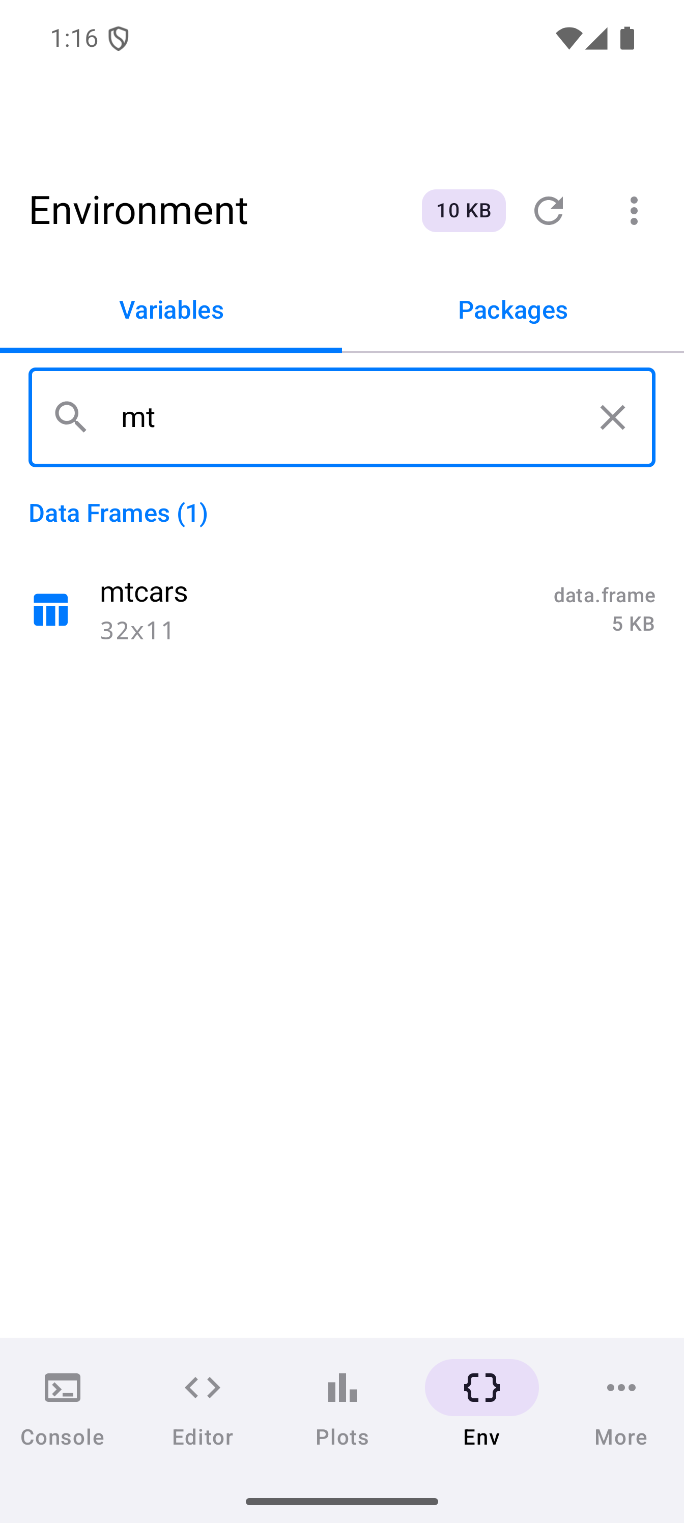
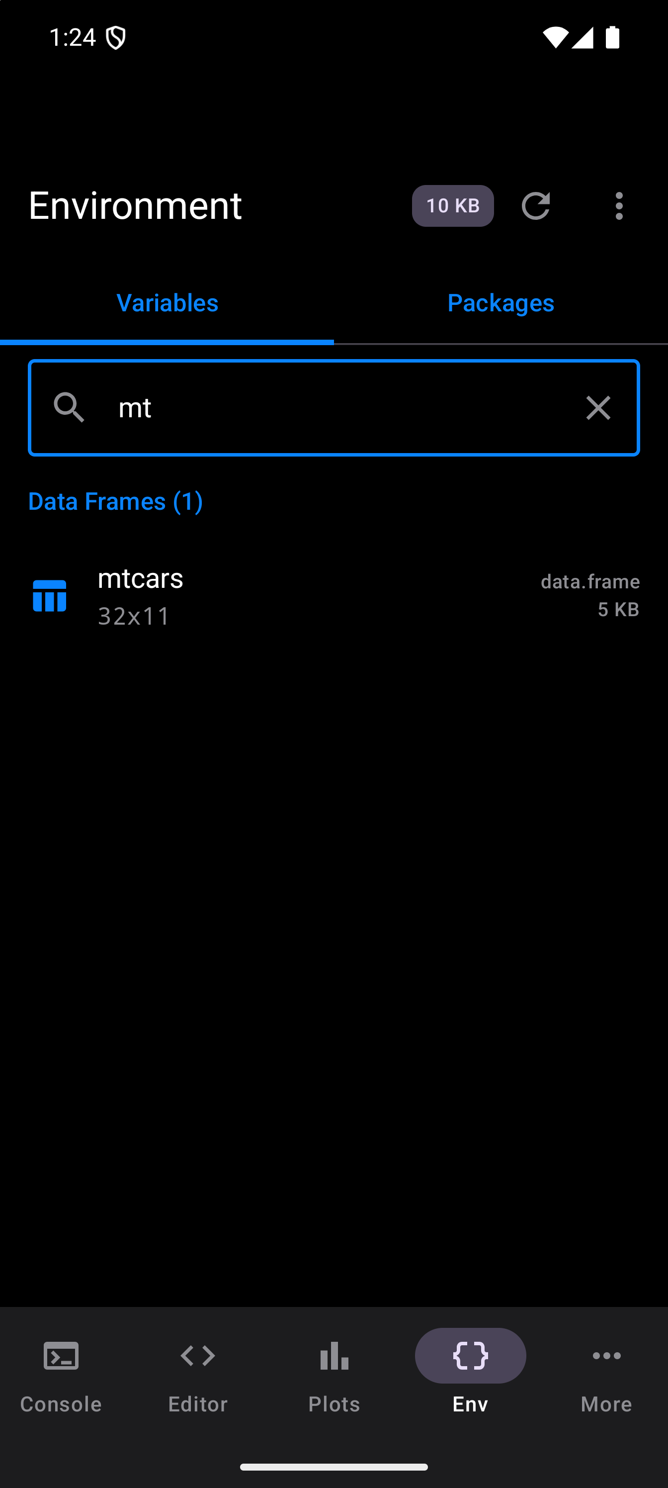
This is faster than scrolling through dozens of entries, especially when you have many similarly named variables.
Packages Tab
The second tab at the top of the Environment screen is Packages. It gives you a quick count rather than a list. A card called Package Summary shows two numbers:
- Installed is every package R has, including the ones that come with R, so it is more than the number you installed yourself.
- Loaded is how many packages are loaded right now. R loads a few of its own when it starts, such as
statsandutils, so you will see some here even before you load any.
The numbers are read from R each time you open the tab.
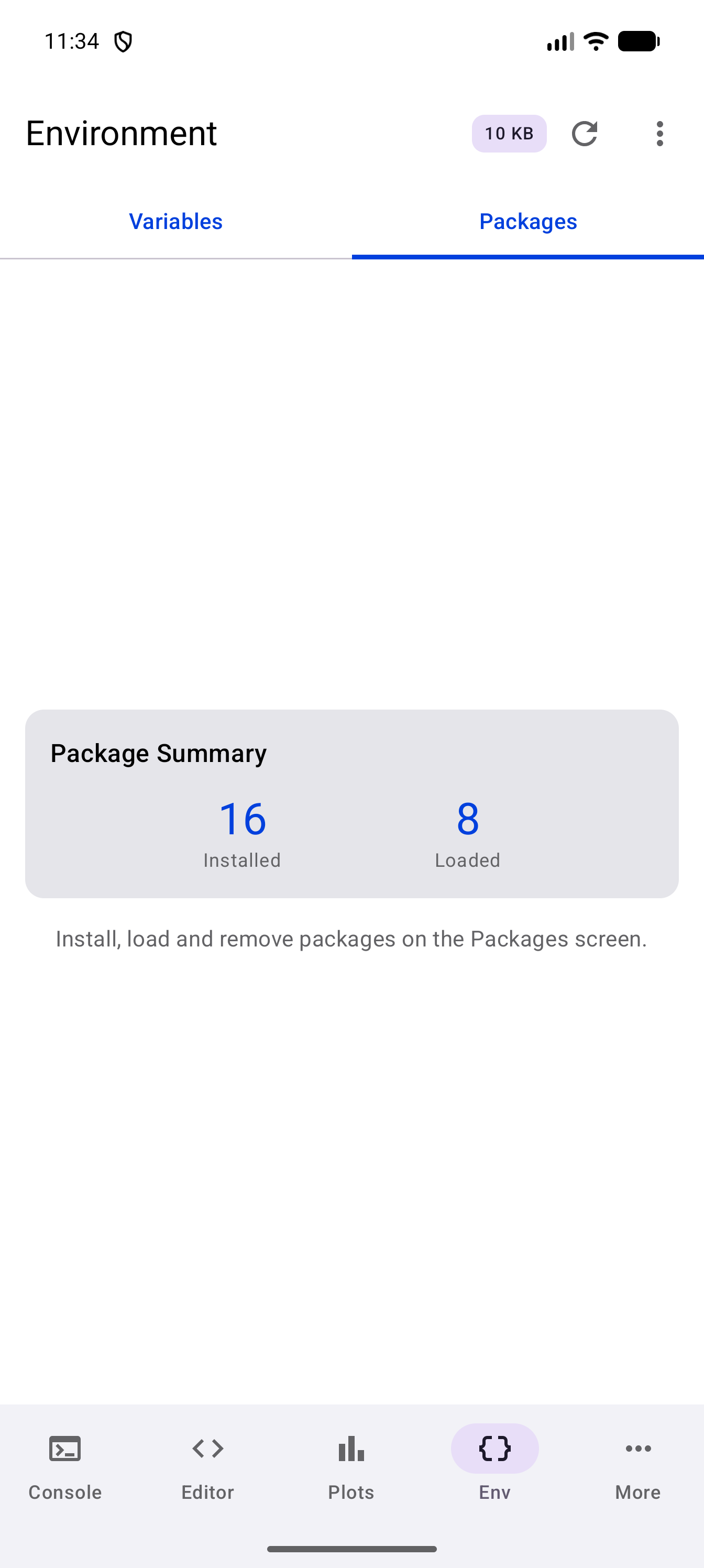
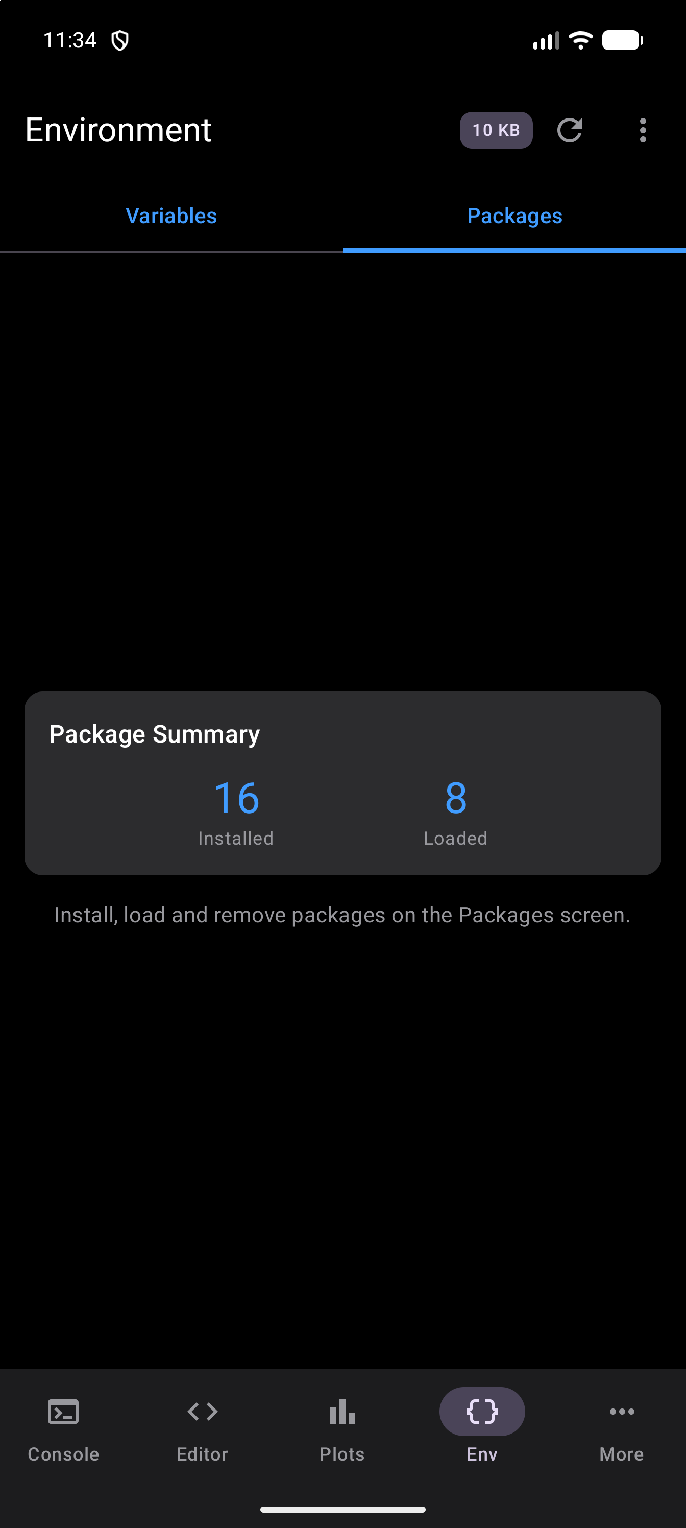
To see the packages themselves, or to install, load, unload or remove one, go to the Packages screen. In the Tab Bar layout, tap More, then Packages. In the Sidebar layout, Packages is right in the sidebar, and in the four-pane Workspace layout on a tablet it is a tab in the bottom-right pane. The line under the card points to that same screen. For more, see the Packages guide.
Environment Menu
The three-dot menu in the Environment title bar has four items:
- Import Dataset… opens Android’s file picker so you can bring a CSV, TSV or Excel file into R as a data frame. See Data Import Wizard.
- Clear Watch List takes every variable off the watch list.
- Clear Environment removes all your variables at once. See Clearing the Environment below.
- Compare Data Frames opens the comparison described in Comparing Data Frames.
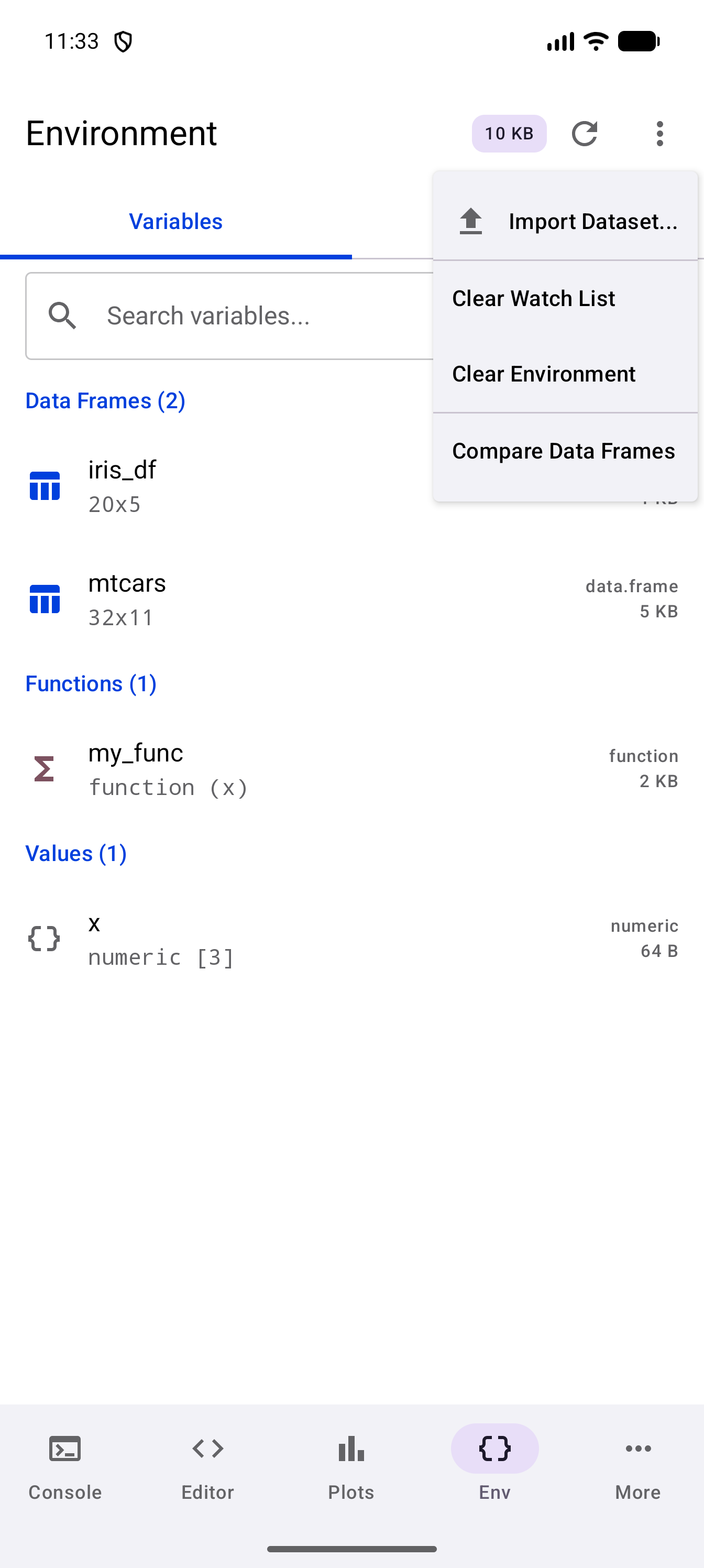
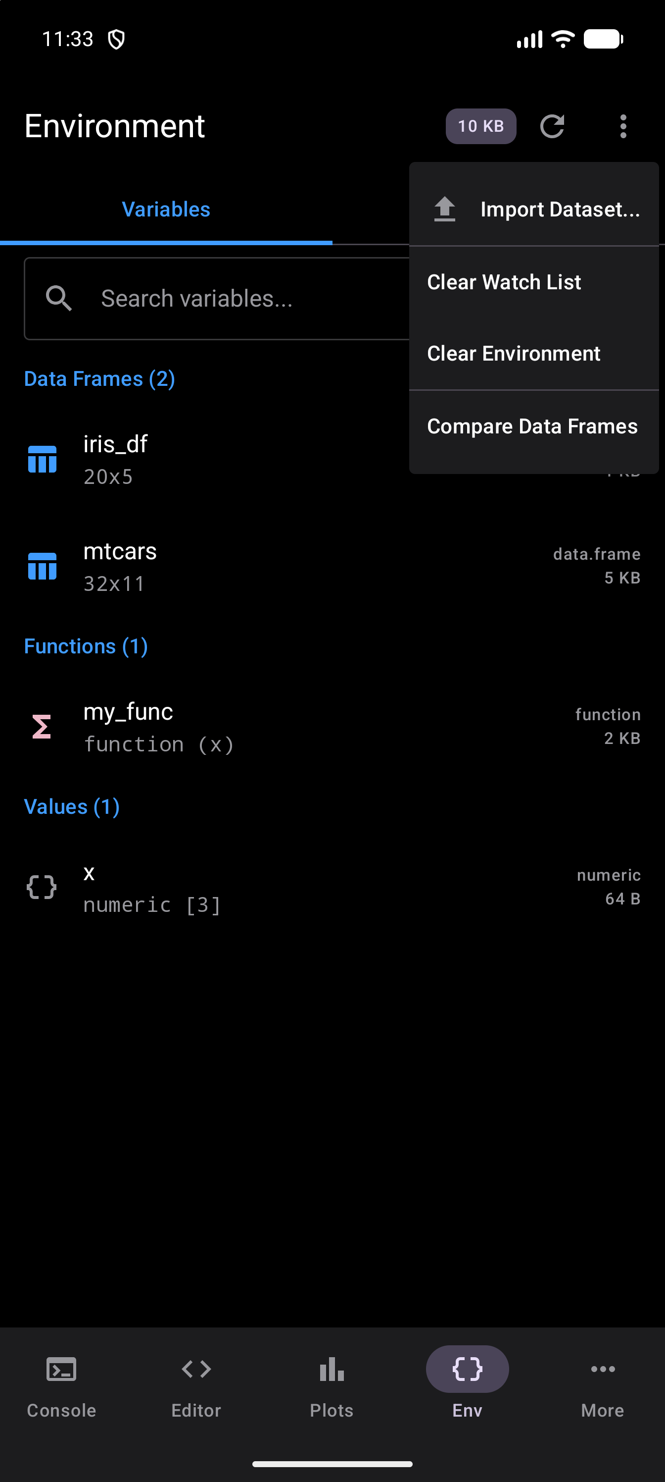
In the four-pane tablet layout, the same menu is in the Environment pane’s header.
Clearing the Environment
Clear Environment removes every variable listed in the Variables tab, whatever its type. It does the same as running rm(list = ls()) in the Console. When it is done, the Variables tab says “No variables in the environment.” and the memory badge shows 0 B.
It does not ask you first, and there is no undo. If there is something you might want back, keep the code that made it in a saved script, so you can run it again.
Only your variables go. Packages you loaded stay loaded, and your files and scripts are not touched. The watch list is left as it is, so if you create a variable again with the same name as one you were watching, it goes straight back into the Watched section.
Memory Tracking
The memory badge in the title bar (e.g., “15 KB”) shows the total memory footprint of your current R workspace. It updates whenever you create, modify, or remove variables.
Each individual variable also displays its own memory size in the list (e.g., “7 KB” for a data frame, “56 B” for a numeric scalar). This helps you identify which objects are consuming the most memory.
Tap the refresh icon in the title bar to read the list and memory figures from R again at once.
If memory usage is climbing and you no longer need certain variables, remove them with rm() in the Console or choose Delete from a variable’s long-press menu, which works on names that need backticks, such as `my data`, too. Large data frames and lists are usually the biggest consumers. To remove every variable at once, use Clear Environment.
Workspace Mode
In the four-pane tablet layout, the Environment appears in a compact workspace mode. The full-size title bar gives way to a slimmer pane header: “Environment” with the memory total beside it, and a Settings gear, the refresh icon and the overflow menu on the right. The content is the same (grouped variables, search, and quick actions), but it is designed to share the screen with the Console, Editor, and other panes.